Science · Code · Curiosity

Gravity
Introduction
By the end of this tutorial we will have a complete simulation of a classical problem in physics: the trajectory of a projectile. In this tutorial, we will:
- Create a function to add vectors
- Create a vector to represent gravity
- Add drag and elasticity
And after that we should have a simulation that looks a bit like this:
As usual the full code can be found by clicking the Github link at the top of the page.
Gravity works by exerting an constant downward force to each of the particles in the simulation. If we had stored the particles' movement as two positions, dx and dy (as discussed here), then we could simply add a constant to the dy value. However, since we’re using vectors, it’s a bit more complex because we need to add two vectors. Once we have a function to add vectors (which took me a while to work out, but is probably the most useful thing in these tutorials), everything else will be a lot easier.
Adding Vectors
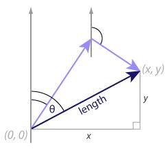
The addVectors() function takes two vectors (each an angle and a length), and returns single, combined a vector. First we move along one vector, then along the other to find the x,y coordinates for where the particle would end up (labelled (x, y) on the diagram below).
def addVectors((angle1, length1), (angle2, length2)):
    x = math.sin(angle1) * length1 + math.sin(angle2) * length2
    y = math.cos(angle1) * length1 + math.cos(angle2) * length2
We then calculate the vector that gets there directly. To do this we construct a right-angle triangle as shown in the image below. Then we use good old trigonometry and a couple of handy functions from Python’s math module, which I’ve only recently discovered.
The new vector length (speed of the particle) is equal to the hypotenuse of the triangle, which can be calculated using math.hypot(). This takes an x,y coordinate and calculates its distance from the origin (0,0). Note that while the position of our particle on the screen is not (0,0), all the vectors are relative to the particle's position, so can be considered to begin at 0,0.
The angle of the new vector is slightly more complex to calculate. First, we find the angle in the triangle, by calculating the arctangent of y/x. We could do this using the math.atan() function but then we would then need to deal with the case of x=0 and work out the sign of angle. However, Python provides us with a handy function math.atan2(), which takes the x, y coordinates, works out the sign of the angle for us and behaves correctly when x=0. Once we have the angle of the triangle, we subtract it from pi/2 to calculate the angle of the vector.
length = math.hypot(x, y)
angle = 0.5 * math.pi - math.atan2(y, x)
return (angle, length)
Gravity
Now we can create a vector for gravity: the angle is pi, which is downward and I chose a magnitude of 0.002 purely by experimentation. Feel free to change it:
gravity = (math.pi, 0.002)Then, in the Particle's move() function, we add the gravity vector to the particle’s vector:
(self.angle, self.speed) = addVectors((self.angle, self.speed), gravity)Friction
To complete the trajectory simulation and stop the particles from bouncing forever we need to add two more physical phenomena: drag and elasticity.
Drag represents the loss of speed particles experience as they move through the air - the faster a particle is moving, the more speed is lost. I find it simpler (and computationally quicker) to define a drag variable that represents the inverse of drag. We multiple a particle's speed by this value at each time unit, thus the smaller the value, the more speed is lost. Elasticity represents the loss of speed a particle experiences when it hits a boundary.
You can play with the values to see what looks reasonable, though both should be between 0 and 1. I found that 0.999 and 0.75 respectively work quite well.
drag = 0.999
elasticity = 0.75
To the Particle's move() function add:
self.speed *= dragAnother option would be to multiply by a factor that varied inversely with the particle's size (e.g. self.speed *= (1-self.size/10000.0)), but I don't think that's necessary.
After each of the four boundary conditions, add:
self.speed *= elasticityself.speed *= elasticityself.speed *= elasticityself.speed *= elasticityAnd there you have it: a complete simulation of a projectile's trajectory. And we haven't had to explicitly solve any of the equations of motion. Try running the simulation several times to see what happens. You might find it easier to set the y coordinate to 20, so the particle always starts at the top of the simulation. In the next tutorial, we add some user interaction so you can pick up, drop and throw the ball (particle).
Comments 15
Leave a comment
Comments are moderated and will appear after approval.
Hello!
Nice tutorials. I learned a lot from them. But one thing. The window doesn't close nicely so what i usually do is that I import pygame like this:
import sys, pygame from pygame.locals import *
and then make the main loop like this:
while True:
for event in pygame.event.get():
if event.type == pygame.QUIT:
pygame.quit()
sys.exit()
Now the window shuts nicely when you press the windows closing button.
(Sorry about the bad english)
I've never had a problem with the window not closing properly. I think the reason you might is that you're using an integrated development environment (IDE). If your code fixes the problem then that's great. I guess it's probably best to call pygame.quit() and sys.exit() just to be on the safe side anyway.
Ok. I am using IDE, so that's the reason then. I'm really new in writing python so I'm not familiar with other options there are available yet.
Peter
Apologies, I just submitted a comment but there were a couple of typo errors. I referred to Tutorial 5 but I meant Tutorial 6 and my code misspelt 'length2' and should have read;
def addVectors(vector1, vector2):
angle1, length1 = vector1
angle2, length2 = vector2
Hope this all makes sense.
Regards
Gary
Hi!
first of all, thank you very much for this tutorial, it's great!
i have a little problem with the behavior of the particles. over time, if not using drag or elasticity, the "energy" of the system is not conserved. i noticed that because i measured the average speeds over time in the beginning and in the end, and it was significally different - its getting higher over time. what can be the source of that?
i tried to deal with this in several ways, but none of them was elegant and accurate enough for my final goal, which is a simulation of a ideal gas in a tank with gravity.
Hi Yigal,
The equation used here is a big simplification and does tend to lead to increased momentum over time. I've you skip to the tutorial on mass, I use a much better equation which should conserve momentum (although there can still be problems because we have to use discrete units of time).
I believe it would be easier if you measured the angle from the positive x-axis counter clockwise. Then you wouldn't have to subtract the result of atan2(y, x) from pi/2
Hey!
These are truly fantastic tutorials that you put together!!! I was wondering how you are choosing the numbers for gravity and so on. Do you have guideline values that can be deducted from the real values (e.g. g = 9.81 etc.)?
Just wondering as I can't see a pattern. Thanks a lot (also for the tutorials)
Thanks. I just picked values that seemed to give a nice result. If you were going to pick real values then you'd have to decide on a scale, so 1 pixel = 1m or something and then you could work out the values from there. Even so, it might be hard to find accurate values or elasticity or resistance in the form that I have it.
Hello from the year 2016! I've been learning a lot from these turtorials I just wanted to say thanks for doing these they are awsome. Now, python has grown a lot over the years and I am now having some trouble translating your code. When I call addVectors in the class function move() the shell keeps saying that it is missing one argument. Now you dont have to answer this but it would be cool!
I copied it the code straight in, but i can't seem to get it to work due to this.
anyone out there to help me out?
"C:\Program Files (x86)\Python35-32\python.exe" "C:/Users/benny/PycharmProjects/circles tutorial/test.py"
File "C:/Users/benny/PycharmProjects/circles tutorial/test.py", line 11
i made it
def addVectors(angle1, length1, angle2, length2):
but now i get this.
File "C:/Users/benny/PycharmProjects/circles tutorial/test.py", line 40, in move
(self.angle, self.speed) = addVectors((self.angle, self.lenght, self.angle), gravity)
AttributeError: 'Particle' object has no attribute 'lenght'
Greetz Geeo
Hi, can't not say thank you enough for this. I am ME student so those math should not be the issues for me. But the best part of your tutorial is that I now can put it in the computer, which feels really awesome.
Hello sir,
Thank you for this wonderful tutorial series.
I was wondering how did you come up with the formula to calculate x and y in add vector method
def addVectors((angle1, length1), (angle2, length2)):
x = math.sin(angle1) * length1 + math.sin(angle2) * length2
y = math.cos(angle1) * length1 + math.cos(angle2) * length2
length = math.hypot(x, y)
angle = 0.5 * math.pi - math.atan2(y, x)
return (angle, length)
i am weak at maths and I can't understand how to think the way in whic I can find x and y based on angle.
Actually the formula for adding vectors does not work properly, or should I say works only when specific conditions are met. What I mean is you cannot use "math.hypot()" when vectors are parallel (e.g. one is pointing upwards (-pi/2) angle and the other downwards (pi/2 angle)), because one cannot construct a triangle from those.
Referring to pygame docs you can use Vector2 class with its methods "from_polar()" and "as_polar()", just remember about conversions between rads and degrees.
https://www.pygame.org/docs/ref/math.html
Correct me if I'm wrong.
@Rico, math.hypot() will work fine under these circumstances. If the vectors are parallel, then either the x or y value will be 0, but that's fine. The function does not need to actually construct a triangle, it just uses Pythagoras's theorem to find the distance.