Science · Code · Curiosity

Boundaries
Introduction
When creating a simulation you will often want to make it bounded, to avoid simulating an infinite region. In this simulation, a realistic, physical solution is to add virtual walls that particles bounce off. In this tutorial, we will:
- Test whether particles have moved out of the window
- Move such particles to where they would have bounced
- Change their direction appropriately
Another solution would be to bend a 2D simulation into virtual torus (ring doughnut shape). We do this my making particles that leave one side of the simulation appear on the opposite side.
Exceeding boundaries
The first thing our bounce() function needs to do is test whether a particle has gone past a boundary. The four boundaries are at:
- x = 0 (the left wall)
- x = width (the right wall)
- y = 0 (the ceiling)
- y = height (the floor)
Since this simulation has discrete steps of time, we unlikely to catch a particle at the exactly point that it 'hits' a boundary, but rather at a point when it has travelled a bit beyond the boundary. If the speed of the particle is low, then the particle is unlikely to have gone much beyond the boundary (the maximum distance it will have exceeded the boundaries is, in fact, equal to its speed).
We could chose to ignore the discrepancy and simply (especially if our simulation is becoming too computationally intense), and simply reflect the particle angle, but we might as well be accurate for now. Therefore, if a particle exceeds a boundary, we first calculate by how much it has exceeded it (which I'll call d).
For example, if the particle's x value is greater than the window's width minus the particle's size (it has gone beyond the right wall), then we calculate d.
d = self.x - (width - self.size)We then reflect the position in the boundary (i.e. bounce it) by setting the x coordinate as below:
self.x = (width - self.size) - dThis simplifies to:
self.x = 2 * (width - self.size) - self.xSo we don't actually need to calculate variable d. Replacing width with 0 calculates the x position when the particle crosses the left wall. The y coordinates can be calculated in a similar way.
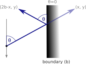
The most important feature of bouncing is reflecting its angle in the boundary, which is where our use of vectors starts to become useful (though its more useful when the boundaries aren't straight). A vertical boundary is has an angle of 0, while a horizontal boundary has an angle of pi. We therefore reflect vertically bouncing particles by subtracting their current angle from 0 and from pi in the case of horizontal bouncing.
The final bounce function should look like this:
def bounce(self):
    if self.x > width - self.size:
        self.x = 2 * (width - self.size) - self.x
        self.angle = - self.angle

    elif self.x < self.size:
        self.x = 2 * self.size - self.x
        self.angle = - self.angle

    if self.y > height - self.size:
        self.y = 2 * (height - self.size) - self.y
        self.angle = math.pi - self.angle

    elif self.y < self.size:
        self.y = 2 * self.size - self.y
        self.angle = math.pi - self.angle
Finally, don't forget to call the bounce() function after calling the move() function and before calling the display() function.
for particle in my_particles:
    particle.move()
    particle.bounce()
    particle.display()
Before running the simulation, I would also increase the width and height to 400 to make things easier to see. When you run this simulation, you should now see ten particles bouncing around at different speeds, but completely ignoring one another. In a later tutorial, we’ll allow the particles to interact with one another.
Comments 21
Leave a comment
Comments are moderated and will appear after approval.
Peter
A superb set of Tutorials. I haven't written any code since Sinclair Basic on the ZX Spectrum. My daughter has expressed an interest in learning to code games and whilst looking at alternative languages I came across your site so I thought Python, Pygame and your physics Tutorials might be a good place to start.
We are using Python 3.2 and have been working through your Tutorials over the couple of evenings. In Tutorial 5 we receive a syntax error in the def addVectors line which appears to be the same syntax error that arose on the second Tutorial relating to 'tuple unpacking'. Whilst not having a clue what tuple unpacking is, we have used the same principle you suggest there and recoded as follows;
def addVectors(vector1, vector2):
angle1, length1 = vector1
angle2, lengthe2 = vector2
This appears to work fine.
Thanks again for sharing your work.
Regards
Gary
Hi Gary,
Thanks for your comment. I also started out programming Basic on the ZX Spectrum. I think programming is a great skill to learn, and coding games is probably the most fun (even if your games are necessarily much simpler than the ones you can buy). I definitely recommend Python as a language to learn programming. You might also want look at inventwithpython.com which goes into a lot more detail.
Hopefully the physics simulation is also a good way to get a more intuitive understanding of physics and mathematics. I certainly gained a much better understanding of what trigonometry was and why it had been invented after working out how to code this simulation.
As for tuple unpacking, a tuple is like a list you can't modify and is convenient for "packing" variables, such as angle and length into a single variable, vector. It seems that in Python 3 they removed the ability to unpack the variables in the parameter list. The way you've solved the problem is correct. One of these days, I'll make the switch to Python 3. I hope it's not too difficult to rewrite what I've done here.
All the best to you and your daughter and good luck with the programming.
Peter
i was wondering about the bounce() method.
do we need to set the "x" value? we could simply could change the direction of the vector when it matches any boundary condition?
Suppose, for right wall the following code works pretty well :
if self.x > width - self.size:
self.angle = - self.angle
Thanks a barrel for your wonderful tutorials :)
just love them :D
Hi Pallab, you can write the code that way if you like, and I often do as it's simpler and realistically doesn't make much difference. In fact, if you remove the code that sets the x and y values, you can reduce the bounce code to two conditionals that check whether either x or y is beyond a boundary.
Hello Peter! I want to thank you for helping me make my future dreams! Great set of tutorials!
Awesome Tutorial.....
nice work...
Peter,
import pygame
import math
import random
(width, height) = (400, 400)
screen = pygame.display.set_mode((width, height))
pygame.display.set_caption("Hello World")
background_colour = (255,255,255)
class Particle:
def init(self, x, y, size, speed, angle):
self.x = x
self.y = y
self.size = size
self.speed = speed
self.angle = angle
self.colour = (0, 0, 255)
self.thickness = 1
def display(self):
pygame.draw.circle(screen, self.colour, (int(self.x), int(self.y)), self.size, self.thickness)
def move(self):
self.x += math.sin(self.angle) * self.speed
self.y -= math.cos(self.angle) * self.speed
def bounce(self):
if self.x > width - self.size:
self.x = 2(width - self.size) - self.x
self.angle = - self.angle
elif self.x < self.size:
self.x = 2self.size - self.x
self.angle = - self.angle
if self.y > height - self.size:
self.y = 2(height - self.size) - self.y
self.angle = math.pi - self.angle
elif self.y < self.size:
self.y = 2self.size - self.y
self.angle = math.pi - self.angle
screen.fill(background_colour)
number_of_particles = 10
my_particles = []
for n in range(number_of_particles): # this loop adds particles with random sizes, speeds, etc
size = random.randint(10, 20)
x = random.randint(size, width - size)
y = random.randint(size, height - size)
a = random.uniform(0, .1) # speed
b = random.uniform(0, 2 * math.pi) #angle
my_particles.append(Particle(x, y, size, a, b))
running = True
try:
while running:
for particle in my_particles:
particle.move()
particle.bounce()
particle.display()
pygame.display.flip()
screen.fill(background_colour)
except SystemExit:
pygame.quit()
Love your tutorials!
I have a question though... I don't quite understand is what 'math.atan2(dy, dx)' is doing exactly. Is it the same as going: 1 / (math.tan(dy/dx))?
Thanks again for the great tutorials.
Leonard
What are the advantages of your method compared to this one : http://pastebin.com/TYmDCS18
Thanks for the answer.
Dear Peter,
Thank you for this impressive tutorial, I found it extremely helpful thus far. Currently, I'm on the Boundaries section where I was slightly confused. It seems as if the speed (how fast the particles move in real time) depend solely on how fast the clock cycles of the computer is (and thus how fast it runs the while statement). In this case, the particle speed becomes pixel/clock cycle rather than pixel/second.
Are my assumptions correct and if so, is the proposed fix I give the most efficient one? If my assumption above is correct then we would run into several issues such as variable speeds for different work stations (this would be bad for gaming). The fix I proposed was to have a cap for the speed, perhaps import that time library and run the loop only every time a set increment of time has passed. This forces the particle to a set speed no matter how fast your computer is.
Also, could you talk a bit more about the math you used to "bounce" the particle?
Best,
Davis
Typo:
"We do this my making particles that leave one side of the simulation appear on the opposite side."
switch my to by
great tutorials btw
Hi Peter,
Thanks so much for these tutorials!
all the best!
Why keep as: self.x = 2*(width - self.size) - self.x
Doesn't that just become: self.x = width - self.size
?
Great working tutorial on Pygame.
I will use this knowledge to further develop my game.
Credits will be given to you!
@gza you're right even I did the calculation. There is a mistake in his subtraction of d.
@gza and @Anshul remember that self.x on the left of the equal sign is going to be the new value of self.x and not the same as self.x on the right side of the equal sign, which is its current value.
For example, say self.x is currently 120, width is 100 and size is 10. In other words, the right hand side of the particle is 30 units past the end of the boundary.
Then:
self.x = 2*(width - self.size) - self.x
self.x = 2 * (100 - 10) - 120
self.x = 2 * 90 - 120
self.x = 180 - 120
self.x = 60
So the right hand side of the particle will be at 70 units (60 + 10), and so 30 units to the left of the boundary.
for people who dont want to have the particles moving at sonic speed
just subtract from the speed when a particle hits a wall.
self.speed -= 0.01
Love your content!
Hi Peter,
Your calculation looks strange and mistaken for me.
self.x = 2 * (width - self.size) - self.x
Example:
w=100
s=20
x=105
self.x = 2*(100-20)-105 = 55 - this result looks wrong for me. I would expect self.x (new) somewhere between 95-100
Hi Roman,
I think the calculation is correct. If the size (radius) of the particle is 20, then the particle should hit the wall at x = 100 - 20 = 80. Instead, it has continued an extra 25 pixels (105 - 80) to the right. Instead of going those extra 25 pixels right from 80, it should have gone left 25 pixels from 80, which is to x = 55.
Still very useful. Thanks!